
Brief Guide on Key Machine Learning Algorithms
Linear Regression
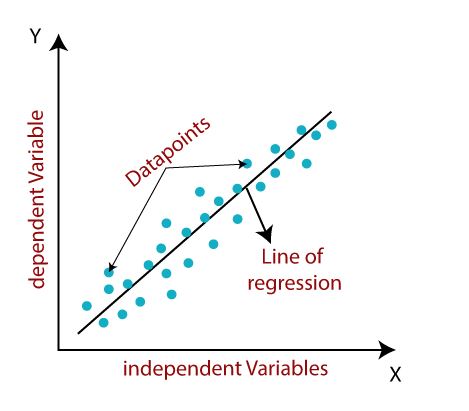
Linear Regression includes finding a ‘line of best fit’ that represents a dataset using the least squares technique. The least squares method involves finding a linear equation that limits the sum of squared residuals. A residual is equivalent to the actual minus predicted value.
To give a model, the red line is a better line of best fit compared to the green line because it is closer to the points, and thus, the residuals are lesser.
Ridge Regression
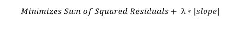
Ridge regression, also identical to as L2 Regularization, is a regression technique that introduces a small amount of bias to reduce overfitting. It is done by minimizing the sum of squared residuals plus a penalty, where the penalty is equal to lambda times the slope squared. Lambda denotes to the severity of the penalty.
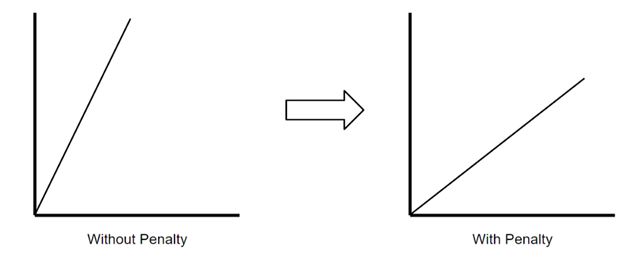
The idea behind ridge regression is that without a penalty, the line of best fit has a steeper slope, which indicates that it is more sensitive to small changes in X. With penalty, the line of best fit becomes less sensitive to small changes in X.
Lasso Regression
Lasso Regression, also referred to as L1 Regularization, is similar to Ridge regression. The only difference is that the penalty is determined with the absolute value of the slope instead.
Logistic Regression
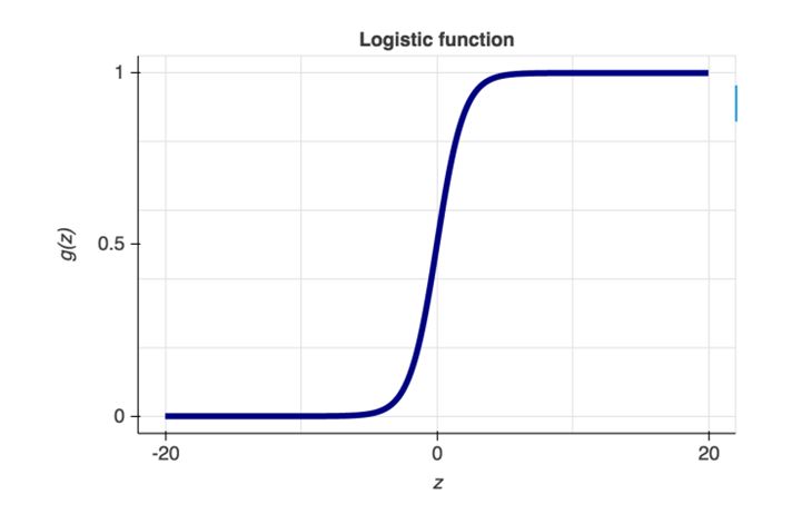
Logistic Regression is a classification technique that also finds a ‘line of best fit.’ However, linear regression finds the line of best fit using least squares, logistic regression finds the line (logistic curve) of best fit by using maximum likelihood. This is due to that y value can only be one or zero
K-Nearest Neighbours
K-Nearest Neighbours is a classification technique, in this a new sample is classified by choosing at the nearest classified points, hence ‘K-nearest.’ In the example below, if k=3, then an unclassified point could be classified as a blue point.
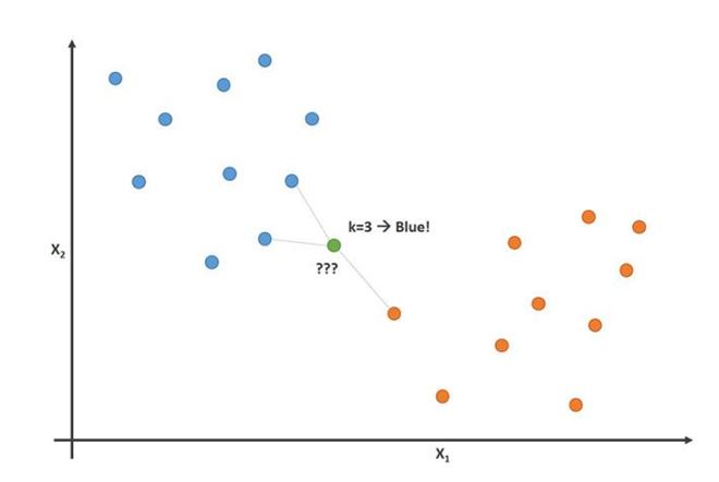
If the value of k is too low, then it leads to outliers. However, if it’s too high, then it might overlook classes with only a few samples.
Naive Bayes
The Naive Bayes Classifier is a classification technique which states the following equation and is inspired by Bayes Theorem:
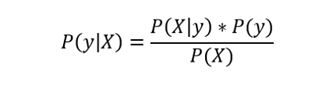
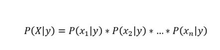
Because of the naive assumption that variables are independent given the class, we can rewrite P(X|y) as follows:
Also, subsequently we are solving for y, P(X) is a constant, this means that we can remove it from the equation and introduce a proportionality.
Hence, the probability of each value of y is determined as the product of the conditional probability of xn given y.
Support Vector Machines
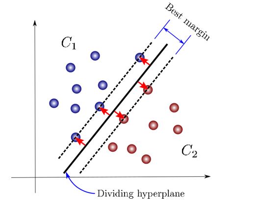
Support Vector Machines are a classification technique that discovers an optimal boundary, called the hyperplane, which is used to separate different classes. The hyperplane is determined by maximizing the margin between the classes.
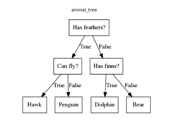
Decision Trees
A decision tree is basically a series of conditional statements that govern what path a sample takes until it reaches the end point. They are intuitive and easy to build yet tend not to be accurate.
Random Forest
Random Forest is an ensemble technique.It combines several models into one to increase its predictive power. Specifically, it builds 1000s of smaller decision trees by utilizing bootstrapped datasets and random subsets of variables (also known as bagging). With 1000s of smaller decision trees, random forests use concept of ‘majority wins’ model to determine the value of the target variable.
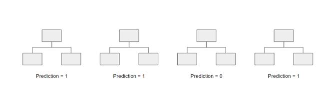
For instance, if we create one decision tree, the third one, it would predict 0. But if we depend on on the mode of all 4 decision trees, then the predicted value would be 1. This is the power of random forests.
AdaBoost
AdaBoost is a boosted algorithm that is alike to Random Forests but has a few significant differences:
- Rather than a forest of trees, AdaBoost typically makes a forest of stumps (a stump is a tree with only one node and two leaves).
- Each stump’s decision is not weighted equally in the final decision. Stumps with less total error (high accuracy) will have a higher say.
- The order in which the stumps are created is important, as each subsequent stump emphasizes the importance of the samples that were incorrectly classified in the previous stump.
Gradient Boost
Gradient Boost is similar to AdaBoost in the sense that it develops multiple trees where each tree is built off of the previous tree. Unlike AdaBoost, which builds stumps, Gradient Boost builds trees with typically 8 to 32 leaves.
More prominently, Gradient Boost differs from AdaBoost in the way that the decisions trees are built. Gradient Boost starts with an initial prediction, generally the average. Then, a decision tree is built depending on the residuals of the samples. A new prediction is made by considering the initial prediction + a learning rate times the outcome of the residual tree, and the process is repeated.
XGBoost
XGBoost is basically the same thing as Gradient Boost, but the main difference lies in how the residual trees are built. With XGBoost, the residual trees are built by determining the similarity scores between leaves and the preceding nodes to fix which variables are used as the roots and the nodes.