Explain different optimization algorithms that we generally use in Neural Network?
Ans: Optimizers are algorithms or methods used to change the attributes of your neural network such as weights and learning rate in order to reduce the losses. There are different types of optimizers, let us see in detail.
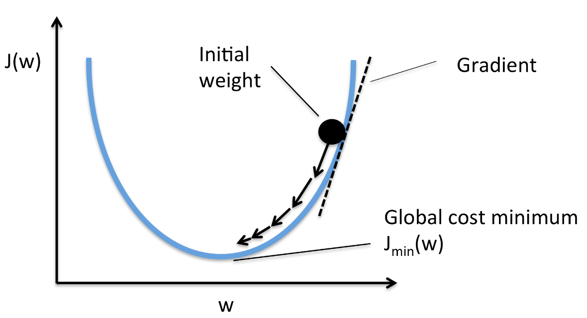
(a)Gradient Descent
Gradient descent is a first-order optimization algorithm. It is dependent on the first order derivative of a loss function. It calculates that which way the weights should be altered so that the function can reach a minima. Through back propagation, the loss is transferred from one layer to another and the model’s parameters also known as weights are modified depending on the losses so that the loss can be minimized.

(b)Stochastic Gradient Descent
It’s a variant of Gradient Descent. It tries to update the model’s parameters more frequently. In this, the model parameters are altered after computation of loss on each training example.
θ=θ−α⋅∇J(θ;x(i);y(i)) , where {x(i) ,y(i)} are the training examples.

As the model parameters are frequently updated parameters have high variance and fluctuations in loss functions at different intensities.
(c) Mini batch Gradient Descent
It’s best among all the variations of gradient descent algorithms. It is an improved on both SGD and standard gradient descent. It updates the model parameters after every batch. So, the dataset is divided into various batches and after every batch, the parameters are updated.

(d) Momentum
Momentum was invented for reducing high variance in SGD and softens the convergence. It accelerates the convergence towards the relevant direction and reduces the fluctuation to the irrelevant direction. One more hyperparameter is used in this method known as momentum symbolized by ‘γ’.
V(t)=γV(t−1)+α.∇J(θ)
Now, the weights are updated by θ=θ−V(t).

(e) Nesterov Accelerated Gradient Descent
If the momentum is too high the algorithm may miss the local minima and may continue to rise up. So, to resolve this issue the NAG algorithm was developed. It is a look ahead method. We know we’ll be using γV(t−1) for modifying the weights so, θ−γV(t−1) approximately tells us the future location. Now, we’ll calculate the cost based on this future parameter rather than the current one.

V(t)=γV(t−1)+α. ∇J( θ−γV(t−1) ) and then update the parameters using θ=θ−V(t).
(f) Adagrad
This optimizer changes the learning rate. It will change the learning rate ‘η’ for each parameter and at every time step ‘t’. It’s a type second order optimization algorithm. It works on the derivative of an error function.

A derivative of loss function for given parameters at a given time t.

Update parameters for given input i and at time/iteration t
η is a learning rate which is modified for given parameter θ(i) at a given time based on previous gradients calculated for given parameter θ(i).
We store the sum of the squares of the gradients w.r.t. θ(i) up to time step t, while ϵ is a smoothing term that avoids division by zero (usually on the order of 1e−8). Without the square root operation, the algorithm does not perform well.

It makes big updates for low frequency parameters and a small step for more frequency parameters.
(g) AdaDelta
AdaDelta is an extension of AdaGrad which tends to remove the decaying learning Rate problem of Adagrad. Adadelta limits the size of the window of accumulated past gradients to some fixed size w. In this exponentially moving average is used rather than the sum of all the gradients.
The value of γ is set around 0.9.


(h) Adam
Adam (Adaptive Moment Estimation) works with momentums of first and second order. The intuition behind the Adam is that we don’t want to roll so fast just because we can jump over the minimum, we want to decrease the velocity a little bit for a careful search. In addition to storing an exponentially decaying average of past squared gradients like AdaDelta, Adam also keeps an exponentially decaying average of past gradients M(t).
M(t) and V(t) are values of the first moment which is the Mean and the second moment which is the uncentered variance of the gradients respectively.

we are taking mean of M(t) and V(t) so that E[m(t)] can be equal to E[g(t)] where, E[f(x)] is an expected value of f(x).
To update the parameter: