Power BI – Pivot Columns

• The Pivot Columns feature in Power Query Editor allows you to transform columns in your data into a pivot table format. This can be useful for analyzing and summarizing data differently, such as comparing data across multiple categories or time periods.
• First, select the columns you want to pivot to use the Pivot Columns feature. Then, select the Pivot Column button in the ribbon. This will open a dialog box where you can specify the column to use as the new pivot column, and any additional aggregation functions you want to perform, such as summing or averaging values.
• Once you have defined your pivot options, click OK to apply the changes. The pivoted data will be displayed in a new table in the Power Query Editor.
• You can further refine the pivoted data by adding additional transformations or calculations. For example, you can create new columns that calculate the difference between different pivot categories, apply additional filters, or sorting to the pivoted data.
• Overall, the Pivot Columns feature in Power Query Editor provides a powerful way to transform and analyze your data in a pivot table format, making it a valuable tool for data professionals and business analysts.

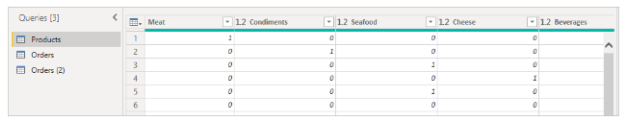
Here’s an example. Each unique product (by name) is listed in the following Products_by_Categories table along with its category. Select the CategoryName column, then select Transform > Pivot Column to create a new table showing each category’s product count.

A dialog box appears letting you know which column values will be used to create new columns. When you expand the Advanced options, you can select the function that will be applied to the aggregated values (if the column name CategoryName isn’t shown).

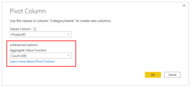
In the Pivot Column dialog box, select OK to display the table based on the transform instructions.