Ridge Regression in Machine Learning
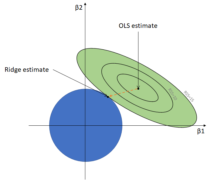
The Ridge Regression is a regularization technique or in simple words it is a variation of Linear Regression. This is one of the method of regularization technique which the data suffers from multicollinearity. In this multicollinearity ,the least squares are unbiased and the variance is large and which deviates the predicted value from the actual value. In this equation also have an error term.
Y=mx+c+error term
Prediction errors are occurred due to bias and variance in this the multicollinearity are reduced by using lamda function.
In Ridge Regression there is no feature selection and it shrinks the value but never reaches to zero. It is also called as L2 regularization technique. Let’s take a dataset and perform the ridge regression ,
The implementation of Ridge regression is:
In this dataset we have 5 columns in which 4 are independent variables and 1 dependent variable.
Import the necessary libraries numpy , pandas , and matplotlib
Import numpy as np

Import pandas as pd

Import  matplotlib.pyplot as plt

%matplotlibinline

Import  sklearn
We can load the data by using read_csv function.
Data=pd.read_csv(“D:\\ML CSV\\classi\\50_Startups.csv”)

Data=pd.read_csv(“path of data.name of data.csv)

Data.head(4)
Output:
| R&D Spend | Adminstration | Marketing Spend | State | Profit |
| 165349.23 | 136897.80 | 471784.10 | Newyork | 192261.83 |
| 162342.63 | 151377.59 | 443898.53 | California | 191792.06 |
| 15344.14 | 101145.55 | 407934.54 | Florida | 191052.06 |
| 144372.65 | 118671.85 | 383199.62 | Newyork | 181765.06 |
By using head function, we can print the first five rows of our data.
Now, we can separate the features and target using iloc function
X=Data.iloc[:,:-2].values

 Y=Data.iloc[:,1:].values

 X

 Y
Here we can train our model by using train_test_split method. We can import this function by sklearn.
from sklearn.model_selection import train_test_split

X_train,X_test,Y-train,Y_test=train_test_split(X,Y,test_size=0.2,random_state=1)
After training we have to fit to our model i.e Ridge regression , for this we can import our model some required parameters mean squared error , r2_score etc.
from sklearn.linear_model import Ridge

from sklearn.metrics import mean_squared_error,r2_score

rr=Ridge(alpha=0,normalize=True,fit_intercept=True)

ridge=rr.fit(x_train,y_train)

ridge
Output:
Ridge(alpha=0, copy_X=True, fit_intercept=True, max_iter=None, normalize=True,random_state=None, solver=’auto’, tol=0.001)
After training, we can predict the test values.
Y_pred=lr.predict(x_test)

 Y_pred
Output:
array([192261.83, 191792.06, 191050.39, 182901.99, 166187.94, 156991.12, 156122.51, 155752.6 , 152211.77, 149759.96, 146121.95, 144259.4 , 141585.52, 134307.35, 132602.65, 129917.04, 126992.93, 125370.37, 124266.9 , 122776.86, 118474.03, 111313.02, 110352.25, 108733.99, 108552.04, 107404.34, 105733.54, 105008.31, 103282.38, 101004.64, 99937.59, 97483.56, 97427.84, 96778.92, 96712.8 , 96479.51, 90708.19, 89949.14, 81229.06, 81005.76, 78239.91, 77798.83, 71498.49, 69758.98, 65200.33, 64926.08, 49490.75, 42559.73, 35673.41, 14681.4 ])
After predicting, we can check the mean_squared_error and r2_score using metrics functions.
mean_squared_error(y_test,y_pred)

r2_score(y_test,y_pred)
Output:
Mean squared error : 77506468.16885379
R2_score : 0.9393955917820573